

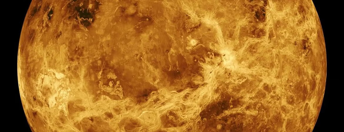
High-performance numerical modeling reveals a narrow path by which a hypothetical Venusian moon could have survived, or been destroyed billions of years ago
Venus presents a unique challenge that traditional observational astronomy cannot resolve: the absence of a natural satellite. This discrepancy prompts a compelling computational inquiry: could Venus have once hosted a significant moon, only to lose it through the complex mechanics of orbital evolution?
A study led by Stephen R. Kane of the University of California, Riverside, in collaboration with researchers from the University of Bordeaux and CNRS, addresses this question as a rigorous numerical experiment. Rather than relying on direct observation, the team developed a computational framework to simulate the evolution of a hypothetical Venus–moon system over billions of years, systematically varying parameters such as planetary rotation, satellite mass, orbital distance, eccentricity, and tidal dissipation. The findings delineate the narrow range of conditions under which such a moon could have survived, while illustrating how the satellite's presence would have fundamentally altered Venus’s rotational history.
The study, titled "Tidal Demise: The Evolution and Fate of a Hypothetical Venus Moon," published in The Astrophysical Journal (https://iopscience.iop.org/article/10.3847/1538-4357/ae9d6c), outlines a semianalytical framework for coupled spin–orbit evolution using two distinct tidal models. For the computational science community, this work reframes the missing moon as a complex reconstruction problem, utilizing numerical integration to determine which initial conditions ultimately led to survival, orbital escape, or catastrophic destruction.
Turning planetary history into a computational problem
The physics begins with a deceptively simple relationship.
A rotating planet exerts tidal forces on an orbiting moon. Those tides exchange angular momentum between the planet’s rotation and the satellite’s orbit.
If Venus rotates faster than the moon orbits, the moon can migrate outward.
But the moon is not merely a passenger.
As it extracts angular momentum from Venus, it also slows the planet’s rotation. That changes the location of the synchronous radius, the orbital distance at which a satellite’s orbital period matches the planet’s rotation period.
The researchers found that this creates a race.
The moon is trying to migrate outward.
Venus’s slowing rotation is causing the synchronous radius to expand outward.
If the synchronous radius catches the moon, the direction of tidal migration can reverse.
The moon can then spiral inward until it reaches the Roche limit, where tidal forces can tear it apart.
The computational problem is therefore a coupled dynamical system rather than a simple orbital calculation.
The study surveys initial Venus rotation periods from 5 to 100 hours, satellite masses from 0.01 to 10 times the mass of Earth’s Moon, initial orbital distances from 3.5 to 25 Venus radii, tidal quality factors from 10 to 100, and orbital eccentricities from zero to 0.5.
That is precisely the sort of parameter-space problem for which numerical computing becomes indispensable.
Instead of asking, “What happens to one hypothetical moon?” the researchers ask a much more powerful question: What happens to thousands of possible Venus–moon systems occupying different regions of physical parameter space?
Two models, two possible futures
The simulations employ two competing descriptions of tidal dissipation.
The first is the constant-Q model, in which the tidal quality factor represents a frequency-independent measure of dissipation.
The second is the constant time lag (CTL) model, in which the deformation of Venus responds with a fixed delay to the tidal forcing.
That distinction becomes particularly important near synchronization.
In the constant-Q model, the tidal torque changes sign discontinuously when Venus’s rotation rate matches the moon’s orbital frequency.
In the CTL model, the torque approaches zero smoothly.
That seemingly technical difference can produce radically different planetary histories.
The CTL model can allow a massive moon to settle into a quasi-synchronous configuration instead of plunging toward destruction. The constant-Q calculation can instead drive the same system through synchronous reversal and eventually into the Roche limit.
For a computational scientist, this is an important reminder that the numerical answer is only as meaningful as the physical model underneath it.
The researchers therefore did not simply run equations and accept whatever came out.
They validated the computational machinery.
The Earth–Moon system becomes the test case
Before trusting the Venus simulations, the researchers applied their integration framework to the Earth–Moon system, where observations provide an unusually valuable benchmark.
Using Earth’s tidal parameters and the Moon’s measured orbital distance, the numerical model reproduced the observed lunar recession rate to within approximately 3 percent.
The calculated value was 3.69 centimeters per year, compared with the observed 3.82 centimeters per year.
The model also reproduced Earth’s changing rotation rate to within approximately 11 percent.
The researchers then performed a much longer numerical experiment, starting Earth with a five-hour rotation period and the Moon at only 3.5 Earth radii.
Using an appropriate time-averaged tidal quality factor, the simulation recovered both the Moon’s present distance of approximately 60.3 Earth radii and Earth’s present approximately 24.5-hour rotation period after 4.5 billion years.
Perhaps more importantly from a computational perspective, the researchers verified angular-momentum conservation to machine precision, with the total spin-plus-orbital angular momentum tracking the expected cumulative solar torque to better than 0.1 percent.
That validation provides confidence that the numerical engine is correctly coupling the planetary spin and satellite orbit before it is unleashed on the far less constrained Venus problem.
The computational machinery
The Venus simulations solve coupled ordinary differential equations describing the evolution of Venus’s spin rate and the satellite’s semimajor axis.
For the CTL calculations, the researchers also employ the full eccentricity-dependent equations developed by Hut and later extended by Leconte and collaborators.
This matters because simplifying eccentricity to a low-order approximation can conceal nonlinear behavior.
The full equations contain eccentricity functions whose terms become increasingly important as eccentricity rises, particularly above approximately e = 0.3.
The coupled equations were integrated using a fourth-order Runge–Kutta method with adaptive timestep control.
The numerical integrator adjusted its timestep so that each step resolved fractional changes of no more than approximately 1 percent in both Venus’s spin rate and the satellite’s orbital distance.
Each simulation was terminated when one of three conditions occurred:
- the satellite crossed the Roche limit;
- the satellite exceeded the critical stability radius;
- or the simulation reached 4.5 billion years.
The calculation also continuously checked angular-momentum conservation.
In other words, this is not a single trajectory plotted on a computer screen.
It is a numerical laboratory for planetary evolution.
Venus turns out to be a very different computational problem from Earth
At first glance, Earth and Venus appear to offer nearly identical starting points for comparison.
They are similar in mass and radius.
But their satellite dynamics are dramatically different.
The researchers found that, in their fiducial Venus system, the moon’s tidal torque on Venus is approximately 3 million times stronger than the solar tidal torque.
That makes the hypothetical moon, not the Sun, the dominant driver of Venus’s early spin evolution.
The reason is partly orbital geometry.
Venus’s smaller Hill sphere means a stable moon must orbit considerably closer to its planet than Earth’s Moon does to Earth.
Tidal torque is extraordinarily sensitive to orbital distance, with the relevant dependence scaling approximately as a⁻⁶.
A small reduction in orbital distance therefore produces a huge increase in tidal interaction.
And that creates a feedback loop.
A closer moon produces stronger tides.
Stronger tides slow Venus more rapidly.
A slower Venus expands the synchronous radius.
The expanding synchronous radius can catch the moon.
And once it does, the moon can begin falling back toward Venus.
The critical race
For the study’s fiducial initial orbital distance of five Venus radii, the moon’s orbital period is approximately 16.1 hours.
That establishes a critical initial Venus rotation period.
If Venus rotates faster than approximately 16.1 hours, the moon begins outside the synchronous radius and initially migrates outward.
If Venus rotates more slowly, the moon begins inside the synchronous radius and immediately spirals inward.
In the constant-Q simulations, a Venus initially rotating once every 24 hours destroys a lunar-mass moon in approximately one million years.
A rapidly rotating Venus produces a very different result.
With an initial rotation period of 8 or 12 hours, a lunar-mass moon initially migrates outward as it extracts angular momentum from Venus. In one representative case, the moon reaches approximately 25 Venus radii before the continuing slowdown of Venus causes the system to reverse direction.
For the one-Moon-mass case, however, that later inward migration is sufficiently slow that the satellite does not reach the Roche limit within the 4.5-billion-year simulation.
The key surprise is that making the moon bigger does not necessarily make it more stable.
It can make the system less stable.
Bigger moon, bigger problem
A two-Moon-mass satellite produces a stronger tidal torque.
That means it can move outward faster.
But it also spins Venus down faster.
And the second effect wins.
At an initial Venus rotation period of eight hours, the constant-Q simulation produces synchronous reversal and eventual Roche destruction at approximately 1.7 billion years for a two-Moon-mass satellite.
At 12 hours, the same mass is destroyed in only about 33 million years.
For a five-Moon-mass satellite, the tidal interaction becomes so powerful that the moon is destroyed within roughly 100 million years, even when Venus begins with a five-hour rotation period.
The mathematical asymmetry is central to the study.
The moon’s outward migration rate scales approximately with its mass.
But the expansion of Venus’s synchronous radius depends more strongly on that mass.
Consequently, increasing satellite mass eventually causes Venus to despin faster than the moon can escape the expanding synchronous region.
The simulation produces a striking diagonal boundary between survival and destruction across the initial-spin/mass parameter space.
This is precisely the sort of nonlinear boundary that is extremely difficult to discover analytically but straightforward to expose computationally through systematic parameter sweeps.
Even eccentricity can rewrite the outcome
The simulations become even more interesting when the researchers allow the moon’s orbit to begin eccentric rather than perfectly circular.
For rapidly rotating Venus, tidal forces can actually pump orbital eccentricity instead of damping it.
The transition occurs around a spin-to-orbital-frequency ratio of approximately 18/11, or 1.636, in the small-eccentricity limit.
For a moon initially five Venus radii away, that corresponds to a Venus rotation period of approximately 10 hours.
The consequence is another computational feedback loop.
A low-mass moon may not exert enough torque to slow Venus quickly.
Venus therefore remains in the eccentricity-pumping regime.
Its moon becomes increasingly eccentric.
Higher eccentricity increases tidal dissipation.
That accelerates orbital evolution and can push the moon toward Venus’s Hill-sphere stability boundary.
The simulation finds that low-mass satellites can be destabilized through this process even when their initial eccentricity is only 0.01.
A sufficiently massive moon can behave differently: its stronger torque rapidly slows Venus below the eccentricity-pumping threshold, after which eccentricity begins to damp.
The computational lesson is profound.
A planetary system’s fate cannot always be inferred from its starting orbital distance alone.
The result depends on the interaction of spin, mass, orbital distance, eccentricity, and tidal rheology, all evolving simultaneously.
The missing moon may not require a missing catastrophe
The simulations ultimately point toward a surprisingly elegant explanation for Venus’s empty sky.
The researchers combine their tidal calculations with recent smoothed-particle hydrodynamics simulations of giant impacts on Venus.
Those impact simulations suggest that scenarios producing Venus’s present-day rotation frequently produce post-impact spin periods of roughly 12 hours or longer, while some impact geometries produce debris disks that remain inside the synchronous orbit and therefore reaccrete onto Venus instead of forming a long-lived moon.
That produces two possible paths.
One possibility is that Venus’s giant impact generated debris but never produced a stable moon in the first place.
The other is more dramatic.
A moon formed, but the coupled gravitational dynamics eventually destroyed it.
The paper finds a particularly interesting tension between these possibilities.
Very rapidly rotating Venus can place a lunar-mass satellite in the survival region, but impact simulations suggest those same conditions may not naturally produce the required long-lived debris disk.
Slower post-impact rotation makes moon destruction more likely.
The authors identify approximately 12–15 hours as a particularly interesting transition region for Venus’s possible last-impact history.
That means the absence of a Venusian moon may be less mysterious than it first appears.
The moon may simply have been a temporary computational state in Venus’s early evolution.
A supercomputer cannot observe the past, but it can test it
There is something deeply inspirational about this kind of computation.
No spacecraft can travel backward four billion years.
No telescope can photograph a moon that may have disappeared before complex life appeared on Earth.
But numerical simulation gives scientists another route.
They can encode the governing physics, establish plausible initial conditions, run the system forward, and determine which histories remain physically consistent with the Venus we observe today.
The result is not a reconstruction of one guaranteed history.
It is a map of possibilities.
And that distinction is important because Venus’s tidal response remains poorly constrained. The planet has no moon whose orbital evolution can be measured directly, leaving considerable uncertainty in its tidal dissipation.
The authors therefore deliberately explore a range of tidal quality factors rather than pretending that one value is known with certainty.
They also emphasize that neither constant-Q nor CTL perfectly represents the complex rheology of a rocky planetary interior. More sophisticated models such as Andrade-type rheologies could place the actual evolution somewhere between the two calculated extremes.
That uncertainty does not weaken the computational approach.
It is precisely why parameter-space exploration matters.
From Venus to exoplanets
Perhaps the most exciting implication reaches far beyond our Solar System.
The researchers suggest that Venus may serve as a natural laboratory for understanding the fate of moons around terrestrial planets orbiting close to their stars.
For planets in the Venus Zone, slow rotation can place the synchronous radius in an unfavorable location, promoting inward satellite migration and eventual destruction.
Around low-mass stars, the situation may become even more extreme because planets receiving Venus-like irradiation must orbit closer to their stars.
Their Hill spheres shrink.
Their moons must orbit closer.
And the powerful distance dependence of tidal torque becomes even more important.
The authors estimate that a Venus analog orbiting at 0.1 astronomical units around a 0.3-solar-mass M dwarf could have a critical spin period roughly 10 times smaller than Venus’s, making long-term survival of a large moon effectively impossible for plausible post-impact rotation states.
That has implications for how astronomers interpret potentially habitable exoplanets.
A planet without a moon may not simply have failed to form one.
It may have formed one, and lost it.
And if a moon influences planetary obliquity, tides, and rotational evolution, losing that satellite could change the long-term climate trajectory of the planet itself.
The next generation of planetary computing
The study also points toward a future in which planetary evolution simulations become increasingly sophisticated.
The present work uses semianalytical tidal models and deliberately explores Venus-specific parameter space. The authors note that atmospheric thermal tides are not included, even though they may play an important role in Venus’s spin evolution.
Adding those effects would likely accelerate the expansion of the synchronous radius and make satellite survival even more difficult.
Future models could couple:
- frequency-dependent planetary rheology;
- atmospheric thermal tides;
- magma-ocean evolution;
- giant-impact simulations;
- debris-disk formation;
- satellite accretion;
- orbital dynamics;
- tidal heating;
- atmospheric evolution; and
- long-term climate models.
That would turn today’s semianalytical experiment into a much larger multiphysics planetary simulation.
And that is where high-performance computing becomes especially powerful.
The ultimate question is no longer simply “Did Venus have a moon?”
It becomes: “What combination of impact physics, planetary interior structure, orbital dynamics, atmospheric tides, and billions of years of nonlinear evolution can produce the Venus we see today?”
Those are questions that cannot be answered with a single equation or a single observation.
They require computation to explore the enormous space between them.
A moon that became a data point
The most profound conclusion from the study by Kane and his colleagues suggests that the absence of a celestial body can serve as a rich source of computational data. The empty orbit around Venus does not inherently imply that no satellite existed; rather, it may represent the terminal state of a dynamical process initiated by a violent planetary collision, wherein gravity and tidal forces gradually obscured all evidence of the moon over billions of years.
The researchers' simulations demonstrate that a lunar-mass satellite orbiting a rapidly rotating Venus could theoretically persist for the entire age of the Solar System. Conversely, minor variations in initial spin, satellite mass, or orbital eccentricity can lead to divergent evolutionary paths. While the boundary between these outcomes is narrow, this is precisely the domain in which computational science excels. Supercomputing does not require prior knowledge of historical events; instead, it allows for the exploration of diverse physical possibilities to determine which scenarios are viable. Ultimately, reconstructing events from billions of years ago begins with a robust set of equations, a rigorous integration loop, and the computational power required to simulate the evolution of the universe.